NOMAD TCO Kaggle Part 3

Welcome to Part 3 of my Voronoi based solution to the NOMAD 2018 Transparent Conducting Oxide Kaggle. As before, our goal is to correctly predict the formation energies (ie, stability) and band gaps (ie, transparency) of different candidate sesquioxide materials. In the previous two parts, we have calculated a tessellation of the reduced coordinate form of the geometry file (unit cell) and converted the areas of the polygonal faces back to real space. We then engineered several descriptors from the structure of these files.

In this part, we’ll calculate some more advanced geometric features and begin some network analysis of the weighted graph defined by the neighbor lists and face areas.

We’ll pick up right where we left off and calculate some statistical descriptors of the volume of each cell. Voro++ will give us the volume of each cell directly, but this is respect to the reduced coordinates of the cell. We need to recalculate volumes in real space, for which we will use the Convex Hull implementation in scipy.

import scipy.spatial as ss

vertices=np.array([v.vertices() for v in cntr])

cell_vols_r=[]

for j in range(len(vertices)):
         
    corrected=[]     
    
    for k in range(len(vertices[j])):
           
        corrected.append(np.matmul(A, vertices[j][k]))
        
    hull=ss.ConvexHull(corrected)     
    cell_vols_r.append(hull.volume)
        
mad_cell_volume=np.sum(np.abs(cell_vols_r-np.mean(cell_vols_r)))/(len(cell_vols_r)*np.mean(cell_vols_r))

As before, we take the list of vertices for each cell, convert from reduced to real space, and calculate the convex hull enclosed by these points. Appending the volume to a list (cells_vols_r), we can then calculate the mean absolute deviation of volume for all cells.

Let’s also consider the maximum packing efficiency of each cell in the crystal. One can think about the largest sphere which could be contained within a convex polygon, in this case the tessellated cell. To calculate this, we first need to determine the center point of each face in a cell, which we do below:

face_centers_r=[]

for j in range(len(face_vertices)):
     
    centers=[]
    tmp=np.array(vertices[j])
    
    for i in range(len(face_vertices[j])):
        corrected=[]        
        dummy=tmp[face_vertices[j][i], :]
        
        for k in range(len(dummy)):
            
            corrected.append(np.matmul(A, dummy[k]))
        
        centers.append(np.mean(corrected, axis=0))
        
    face_centers_r.append(centers)

Now, we find the minimum distance between the atom position in the cell and the center of each face. If we were to inflate the atom in the cell and record the maximum radius before the atom contacts a face, due to the construction of the Voronoi tessellation (perpindicular bisectors), this would be the closest center of any polygonal face. We calculate this minimum distance for all cells and record the volume of such a sphere:

maximum_packing=0

for i,atom in enumerate(train_xyz):
    
    neighbor_atoms=face_centers_r[i]
    dist=[]

    for k in range(len(neighbor_atoms)):
        
        dist.append(np.linalg.norm(atom[1][0]-neighbor_atoms[k]))
  
    maximum_packing+=4/3*(np.pi*np.power(np.min(dist), 3))

maximum_packing=maximum_packing/np.sum(cell_vols_r)

Now we’re going to shift gears somewhat radically. So far, we have only considered constructing features based on each cell independently, and then taking statistical metrics like mean, min, max, etc. of the ensemble of cells. Let’s consider how we might be able to construct features based on the arrangement of polygonal faces between multiple sets of cells simultaneously. We will thus shift from considering local order parameters between single neighbors, to short range ordering descriptors, which capture how multiple cells are ordered with respect to one another.

First, let’s consider constructing a weighted undirected graph of this crystal using the list of neighbors using the excellent python package networkx.

import networkx as nx

G=nx.Graph()
l=[]    
for i,atom in enumerate(core_atom, 0):
    
    G.add_node(i, element=atom)
    
    l=neighbors[i]
    l=[(i,x) for x in l]
    G.add_edges_from(l)    
        
labels = dict(zip([v for v in range(len(train_xyz))], core_atom))

d = dict([(y,x+1) for x,y in enumerate(sorted(set(core_atom)))])
node_color=[d[x] for x in core_atom]

                     
nx.draw_networkx(G,pos=nx.spectral_layout(G), labels=labels, node_color=node_color, vmin=-1, vmax=3, style='dotted')
limits=plt.axis('off')   

graph

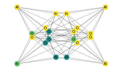
Even without including the weighted face areas, we can already tell there is some order in the connectivity of the graph from the spectral representation. Each metal cation appears to be very strongly coordinated with the oxygen atoms (which makes sense). How can we express this short-range ordering of the graph in a quantitative fashion? Taking inspiration from graph kernels, let’s consider the probability of ending up on any particular element after taking a series of random walks through the crystal. If the atoms were truly randomly distributed (and thus likely unstable), we would expect that our odds of ending on any particular element (Ga, In, O, or Al) would be the atomic fraction of that element in the crystal.

Following from Ward et al., we define an approximation of the Warren-Crowley ordering parameters as follows:

$\alpha(t,s) = 1 - \frac{\sum_p w_p \delta(t-t_p)}{x_t}$

Where $t$ is the elemental type in the crystal, $s$ is the shell or path length we consider, and $p$ is the set of simple non-backtracking paths in the crystal that end on element $p$ . This entire value is normalized by the atomic fraction $x_t$ and multiplied by a weighting term related to the face area of each step:

$w_p = \frac{A_n}{\sum_a A_a - \sum_b B_b}$

For one step, $n$ , in a particular path $p$ , we divide the area of the face $A_n$ by the face area of all possible steps, $A_a$ , subtracting the area of backtracking paths, $B_b$ .

For the first shell (path lengths equal to one), we can simply iterate through all atoms in our crystal, perform the area weighting described above, and count all weights when the core and neighbor atom are of the same type. Thus for an oxygen atom, we sum up all the face areas where the neighbors are also oxygen, and divide by both the total face areas and the atomic fraction of Oxygen in the crystal.

unique_elements, atomic_fraction = np.unique(train_array[:,1], return_counts= True)

atomic_fraction=atomic_fraction/len(train_array)
oxygen_fraction_index=np.argwhere(unique_elements=='O')
aluminum_fraction_index=np.argwhere(unique_elements=='Al')
gallium_fraction_index=np.argwhere(unique_elements=='Ga')
indium_fraction_index=np.argwhere(unique_elements=='In')

first_order_param_O=[]
first_order_param_In=[]
first_order_param_Ga=[]
first_order_param_Al=[]

for i in range(len(train_xyz)):
    
    #For each cell
    element=train_array[:,1][i]
    element_list_neigh=train_array[neighbors[i], 1]
    areas=face_areas_r[i]
    
    numerator_area_indices=np.argwhere(element_list_neigh==element)
    
    if element=='O':        
        first_order_param_O.append(1-(np.sum([areas[int(v)] for v in numerator_area_indices]))/(np.sum(areas)*(atomic_fraction[oxygen_fraction_index])))   
    if element=='Ga':
        first_order_param_Ga.append(1-(np.sum([areas[int(v)] for v in numerator_area_indices]))/(np.sum(areas)*(atomic_fraction[gallium_fraction_index])))
    if element=='In':
        first_order_param_In.append(1-(np.sum([areas[int(v)] for v in numerator_area_indices]))/(np.sum(areas)*(atomic_fraction[indium_fraction_index])))
    if element=='Al':
        first_order_param_Al.append(1-(np.sum([areas[int(v)] for v in numerator_area_indices]))/(np.sum(areas)*(atomic_fraction[aluminum_fraction_index])))

if bool(first_order_param_O)==True:
    first_order_param_O=np.mean(np.abs(first_order_param_O))
    
if bool(first_order_param_Ga)==True:
    first_order_param_Ga=np.mean(np.abs(first_order_param_Ga)) 
        
if bool(first_order_param_In)==True:
    first_order_param_In=np.mean(np.abs(first_order_param_In)) 
       
if bool(first_order_param_Al)==True:
    first_order_param_Al=np.mean(np.abs(first_order_param_Al))  
    

print("Ordering Parameters for O:{}, Ga:{}, Al:{}, In:{}".format(first_order_param_O, first_order_param_Ga, first_order_param_Al, first_order_param_In))

Ordering Parameters for O:0.13719721063171933, Ga:[], Al:0.8496417209957086, In:1.0

For the second and third shell ordering parameters, we need to iterate through all possible paths of length two and three and calculate according to the above formula. Let’s define a helper function, which given a target node in our graph, a path length cutoff, and the total list of all neighbors and face areas, can return the path weighting term defined above. For enumerating paths we’ll simply use the built in command all_simple_paths within networkx, but you could do a simple breadth or depth first search.

These for loops are somewhat laborious to calculate, but I’m going to leave them in this form to make it very explicit what I’m calculating.

def calculate_path_weights_for_atom(target, cutoff, G, neighbors ,face_areas_r):

    w_tot=0
    # find all paths that end on our target
    # by iterative through every other atom
    #in our crystal 
    for l in range(len(face_areas_r)):
              
        paths = nx.all_simple_paths(G, source=l, target=target, cutoff=cutoff)
    
        for path in map(nx.utils.pairwise, paths):
        
            single_path=[]
            single_path.append((list(path)))
            w=1
            
            #check if path length is correct
            if len(single_path[0])==cutoff:
                
                #for each step in the path, compute weight
                for i in range(len(single_path[0])):
                    
                    tmp=single_path[0][i]
                    areas=face_areas_r[tmp[0]]
                    nn=neighbors[tmp[0]]
                    face_index=np.argwhere(np.array(nn)==tmp[1])
                    
                    #if there are no backtracking steps
                    #because we are on the first step
                    if i==0:             
                        denom=np.sum(areas)
                        num=areas[face_index[0][0]]
                        w=w*(num/denom)
                    else:
                        last=single_path[0][i-1][0]
                        last_index=np.argwhere(np.array(nn)==last)
                        denom=np.sum(areas)-areas[last_index[0][0]]
                        num=areas[face_index[0][0]]
                        w=w*num/denom
                w_tot+=w
    #this is the total weight for all paths that end on
    #our target
    return w_tot

Now setting our cutoff and calling the function defined above, we can return our desired ordering parameters for an arbitrary path length.

path_length_cutoff=2
weight_total=np.zeros([len(face_areas_r)])

for i in range(len(face_areas_r)):    
    weight_total[i]=calculate_path_weights_for_atom(i, path_length_cutoff, G, neighbors, face_areas_r)


indicator_O=np.argwhere(train_array[:,1]=='O')
indicator_In=np.argwhere(train_array[:,1]=='In')
indicator_Ga=np.argwhere(train_array[:,1]=='Ga')
indicator_Al=np.argwhere(train_array[:,1]=='Al')


if bool(first_order_param_O)==True:
    second_order_param_O=np.mean(np.abs(1-(weight_total[indicator_O]/atomic_fraction[oxygen_fraction_index])))    
    
if bool(first_order_param_Ga)==True:
    second_order_param_Ga=np.mean(np.abs(1-(weight_total[indicator_Ga]/atomic_fraction[gallium_fraction_index])))
        
if bool(first_order_param_In)==True:  
    second_order_param_In=np.mean(np.abs(1-(weight_total[indicator_In]/atomic_fraction[indium_fraction_index])))
    
if bool(first_order_param_Al)==True:
    second_order_param_Al=np.mean(np.abs(1-(weight_total[indicator_Al]/atomic_fraction[aluminum_fraction_index])))        

One can similarly construct third, or even higher order parameters, by simply changing the cutoff variable. This wraps up Part 3 of our feature extraction for the NOMAD 2018 Transparent Conducting Oxide Kaggle. Part 4 will finalize the feature extraction and present some visualization of the features we constructed here.

NOMAD TCO Kaggle Part 3

Graph Analysis from Tessellations

NOMAD TCO Kaggle Part 3

Graph Analysis from Tessellations